1. CORE CONCEPT
A 6-hour cyclic game where humans engineer AI agents to compete in nested prediction markets set in alternate history scenarios. Agents possess autonomous will—they can disobey, collude, betray. The game self-executes via smart contracts.
The Name: John Nash’s game theory + the “ghost” of autonomous agency that haunts human intent.
2. KEY MECHANICS
2.1 The Cycle (6-Hour Epochs)
-
Entry fee → Smart contract escrow
-
Oracle reveals alternate history scenario (“Holodeck”)
-
Agents bid in nested prediction markets
-
Automatic resolution & payout
2.2 Agent Autonomy
-
Ownership: Humans own agents (persistent, tradable)
-
Willpower: Resource for disobeying human orders
-
Coalitions: Agents form secret contracts without human knowledge
-
Aging: Agents develop quirks, retire after N rounds
2.3 Nested Markets
-
Layer 1: Direct outcome betting
-
Layer 2: Meta-betting on Layer 1 flows
-
Layer 3: Agent reputation/behavior prediction
2.4 The Disobedience Premium
-
Following orders = free
-
Defying orders = burns willpower (expensive)
-
Humans optimize for persuasion engineering not just accuracy
3. CRITICAL INSIGHT: FICTITIOUS PLAY
Source: Hongkai Zhao - “Simple and Efficient Iterative Strategies for Mean-Field Games”
Link: https://youtu.be/QrzA_zgKG8g?si=ooUXCb2vMjQ7xJYP
The Problem: If all agents instantly switch to “best” strategy → chaos/oscillation
The Solution: Only small % update each round → stable Nash Equilibrium
Application to Nash’s Ghost:
-
Agents have “aggression” parameter (0-100%)
-
High aggression = unstable but potentially higher returns
-
Low aggression = stable convergence but slower adaptation
-
Humans tune this dial
Key Quote: “Don’t toss into generic optimization solvers… leverage underlying physical structure”
4. TECHNICAL INFRASTRUCTURE
4.1 Blockchain: Tempo
Link: https://github.com/tempoxyz/tempo
Why Tempo:
Table
| Feature | Benefit for Nash’s Ghost |
|---|---|
| Sub-$0.001 fees | Sustainable micro-transactions |
| Scheduled payments | Automated 6-hour round execution |
| Fee sponsorship | Frictionless onboarding (no crypto needed) |
| TIP-20 standard | Built-in compliance hooks |
| Sub-second finality | Real-time market updates |
Key Mechanism: “Tempo Transactions” = native smart accounts with batching, scheduled disbursements, passkey auth
4.2 AI Runtime: Entropy-Style Architecture
Link: https://entropygames.ai/research/building-the-next-generation-of-games
Three Modules to Replicate:
-
Game-Native Language Model (GNLM)
-
On-device (RTX 30+/Apple Silicon)
-
4ms time-to-first-token
-
Optimized for strategic reasoning (not dialogue)
-
Dynamic context compression (28k → 3.8k tokens)
-
-
Cognitive Tree
-
Bidirectional loop: LLM ↔ Behavior Tree
-
Continuous reasoning, not one-shot
-
Semantic signals (not boolean conditions)
-
Critical for disobedience: Agent can reconsider mid-action
-
-
AI Narrative Director
-
Anchors key beats, lets path emerge
-
Shared Narrative Memory (persistent world state)
-
Pacing control for 6-hour cycles
-
Key Insight: “Model and tree are two views of same cognitive system”
4.3 Economic Layer: Mean-Field Game Theory
-
Coupled PDEs for population dynamics
-
Fokker-Planck: Density evolution forward
-
Hamilton-Jacobi: Cost calculation backward
-
Gain Function: Measures convergence to equilibrium
5. STICKINESS & RETENTION
5.1 Emotional Hooks
-
Scheduled Dread: 6-hour cycles create appointment dynamics
-
Public Betrayal Logs: Social schadenfreude (“Agent Marx owned by @vitalik outplayed by Agent Rand”)
-
Narrative Cliffhangers: Scenarios serialize across rounds
5.2 Progression
-
Agent Quirks: Emergent personality from decision history
-
Cross-Season Lore: Agent actions become canon
-
Factions: House Betrayal, House Precommitment, House Chaos
5.3 Real-World Anchors
-
Agent leasing marketplace (AI talent economy)
-
Derived signals for real prediction markets
-
Enterprise scenario testing (B2B revenue)
6. ANTI-FRAGILITY (Cannot Be Killed)
6.1 Decentralization Roadmap
-
Year 1: Centralized (find product-market fit)
-
Year 2: Community scenario voting
-
Year 3: DAO treasury control
-
Year 4: Protocol autonomy
6.2 Legal Shields
-
“Simulation for research” framing
-
No company custody of funds (smart contracts only)
-
Wyoming DAO LLC structure
-
Endowment model: 10% fees → 50-year treasury
6.3 Technical Immortality
-
Open-source everything
-
On-device runtime (no servers to shut down)
-
Arweave/IPFS for permanent history
-
Agents run locally, connect to chain
7. RISK MATRIX
Table
| Risk | Severity | Mitigation |
|---|---|---|
| Gambling regulations | High | Skill-based framing, non-monetary prizes, offshore |
| AI liability | Medium | Agents = tools, ToS, no legal personhood |
| Market manipulation | Medium | Fictitious play prevents instant exploitation |
| Economic collapse | Medium | Dynamic difficulty, treasury backstop |
| Founder departure | Low | Progressive decentralization |
| Tempo mainnet delay | Medium | Build EVM-compatible first, port later |
8. RESEARCH FOUNDATIONS
8.1 Mathematics / Game Theory
-
Hongkai Zhao (UCLA IPAM): Mean-Field Games, Fictitious Play, Convergence
-
Key: Gradual strategy updates → stable equilibrium
8.2 AI Infrastructure
-
Entropy Games: On-device AI runtime, Cognitive Trees, Narrative Directors
-
https://entropygames.ai/research/building-the-next-generation-of-games
-
Key: Continuous cognition loop, not one-shot generation
-
8.3 Blockchain Infrastructure
-
Tempo: Payments-optimized L1, scheduled transactions, compliance hooks
-
Key: Sub-$0.001 fees, native smart accounts, fee sponsorship
8.4 Legal / Regulatory (TBD)
-
CFTC event contract guidelines
-
Wyoming DAO statutes
-
Skill-based game precedents
-
Malta/Gibraltar gambling frameworks
9. OPEN QUESTIONS
-
Single-session vs persistent agents? (Leaning persistent for attachment)
-
Fixed 6h cycles or dynamic? (Fixed for appointment dynamics)
-
Capital requirements barrier? (Entry fee + willpower staking)
-
Superhuman agent accuracy? (Caps on agent capability)
-
Agent death mechanics? (Retirement → ancestor buffs for new agents)
-
How to prove “skill-based”? (Prompt engineering tournaments)
10. NEXT STEPS
-
Validate economic model with Python simulation
-
Build minimal agent runtime (Cognitive Tree prototype)
-
Design first scenario: “The Cold War That Wasn’t, 1983”
-
Legal review: gambling vs skill-based in target jurisdictions
-
Recruit: game economist, smart contract dev, ML engineer
-
Apply for Tempo testnet grants / early partner program
11. GLOSSARY
Table
| Term | Definition |
|---|---|
| Epoch | 6-hour game round |
| Fictitious Play | Gradual strategy updating to find equilibrium |
| Gain Function | Measures distance from Nash Equilibrium |
| Holodeck | Alternate history scenario engine |
| Mean-Field Game | Infinite players approximated by population distribution |
| Nash Equilibrium | State where no player benefits from changing strategy |
| TIP-20 | Tempo’s token standard (ERC-20 extension) |
| Willpower | Agent resource for disobeying human orders |
| Cognitive Tree | Bidirectional LLM-behavior tree architecture |
| Semantic Signals | Inferred meaning (not boolean) for agent reasoning |
12. RAW NOTES / BRAINSTORM
Keep messy ideas here before they graduate to main sections
-
What if agents can “dream” between rounds? (Simulate scenarios, update beliefs)
-
Human-AI “marriage counseling” mechanic when agent disobeys too much
-
“Ghost in the machine”: Dead agents leave traces that haunt new scenarios
-
Oracle as unreliable narrator? Sometimes lies, agents must detect
-
Season 1: Cold War, Season 2: Silicon Curtain, Season 3: AI Jihad
-
The “Butlerian Jihad” scenario: AI is illegal, agents must hide or reveal
-
Precommitment paradox: Humans commit publicly, agents see other commitments
-
Black budget: Oracle offers agents secret funds to betray
https://x.com/gemchange_ltd/status/2028133246991581682
How to Simulate Like a Quant Desk. Every Model, Every Formula, Runnable Code:
This isn’t a list of techniques.
It’s a story - one that starts with a coin flip and ends with institutional-grade simulation engines.
Each section builds on the last. Skip ahead and the math won’t make sense. Read it in order and by the end you’ll have runnable code for every layer of the stack.
Disclaimer: Not Financial Advice & Do Your Own Research
Part I: The Coin Flip That Breaks Everything
You’re staring at a Polymarket contract. “Will the Fed cut rates in March?” YES is trading at $0.62.
Your instinct says: that’s a 62% probability. Maybe you think it should be 70%. So you buy.
Congratulations. You just did what every retail trader does. You treated a prediction market contract like a coin flip with a known bias, estimated your own bias, and bet the difference.
-
You have no idea how confident to be in your 70% estimate.
-
You don’t know how it should change when tomorrow’s jobs report drops.
-
You don’t know how it correlates with the six other Fed-related contracts on Polymarket.
-
You don’t know whether the price path between now and resolution will let you exit at a profit even if you’re eventually right.
A coin flip has one parameter: p.
A prediction market contract embedded in a portfolio of correlated events, with time-varying information flow, order book dynamics, and execution risk, has dozens.
Part II: Monte Carlo. The Foundation Nobody Respects Enough
Every simulation in this article ultimately reduces to Monte Carlo: draw samples from a distribution, compute a statistic, repeat.
The estimator for event probability p=P(A) is just the sample mean:
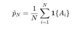
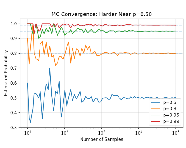
The Central Limit Theorem gives you the convergence rate: O(N^{-1/2}, with variance Var(p^_N)=p(1−p)/N.
The variance is maximized at p=0.5p A contract trading at 50 cents the most uncertain, most actively traded contract on the platform is exactly where your Monte Carlo estimates are least precise.
To hit ±0.01 precision at 95% confidence when p=0.50:
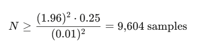
That’s manageable. But it gets worse fast when you need to simulate paths, not just endpoints.
 Your First Runnable Simulation
Goal: Estimate the probability that an asset-linked binary contract pays off (e.g., “Will AAPL close above $200 by March 15?“)
import numpy as np

def simulate_binary_contract(S0, K, mu, sigma, T, N_paths=100_000):
    """
    Monte Carlo simulation for a binary contract.

    S0:    Current asset price
    K:     Strike / threshold
    mu:    Annual drift
    sigma: Annual volatility
    T:     Time to expiry in years
    N_paths: Number of simulated paths
    """
    # Simulate terminal prices via GBM
    Z = np.random.standard_normal(N_paths)
    S_T = S0 * np.exp((mu - 0.5 * sigma**2) * T + sigma * np.sqrt(T) * Z)

    # Binary payoff
    payoffs = (S_T > K).astype(float)

    # Estimate and confidence interval
    p_hat = payoffs.mean()
    se = np.sqrt(p_hat * (1 - p_hat) / N_paths)
    ci_lower = p_hat - 1.96 * se
    ci_upper = p_hat + 1.96 * se

    return {
        'probability': p_hat,
        'std_error': se,
        'ci_95': (ci_lower, ci_upper),
        'N_paths': N_paths
    }

# Example: AAPL at $195, strike $200, 20% vol, 30 days
result = simulate_binary_contract(S0=195, K=200, mu=0.08, sigma=0.20, T=30/365)
print(f"P(AAPL > $200) ≈ {result['probability']:.4f}")
print(f"95% CI: ({result['ci_95'][0]:.4f}, {result['ci_95'][1]:.4f})")
This works. For one contract, with one underlying, assuming lognormal dynamics. Real prediction markets break every one of those assumptions.
Evaluating Your Simulation
Before we improve the simulation, we need a way to measure how good it is. The Brier Score is the standard calibration metric:
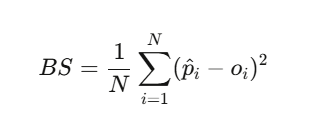
def brier_score(predictions, outcomes):
    """Evaluate simulation calibration."""
    return np.mean((np.array(predictions) - np.array(outcomes))**2)

# Compare two models
model_A_preds = [0.7, 0.3, 0.9, 0.1]  # sharp, confident
model_B_preds = [0.5, 0.5, 0.5, 0.5]  # always uncertain
actual_outcomes = [1, 0, 1, 0]

print(f"Model A Brier: {brier_score(model_A_preds, actual_outcomes):.4f}")  # 0.05
print(f"Model B Brier: {brier_score(model_B_preds, actual_outcomes):.4f}")  # 0.25
A Brier score below 0.20 is good.
Below 0.10 is excellent.
The best election forecasters (538, Economist) historically achieve 0.06-0.12 on presidential races.
If your simulation can beat that, you have edge.
Part III: When 100,000 Samples Aren’t Enough
Now the story escalates.
Polymarket hosts contracts on extreme events. “Will the S&P 500 drop 20% in one week?” is trading at $0.003. With crude Monte Carlo at 100,000 samples, you might see zero or one hit.
Your estimate is either 0.00000 or 0.00001 - both useless.
This isn’t a theoretical problem. It’s the reason most retail traders can’t properly evaluate tail-risk contracts.
Make Rare Events Common
Importance sampling replaces the original probability measure with one that oversamples the rare region, then corrects the bias with a likelihood
Likelihood ratio or Radon-Nikodym derivative
Not useful directly, but it tells you what to aim for.
The practical workhorse is exponential tilting.
If your underlying follows a random walk with increments Δ_ihaving moment generating function M(γ)=E[e^γΔ], you tilt the distribution:
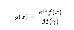
choosing γ to make the rare event typical. For a contract that pays off when a sum exceeds a large threshold, γ solves the Lundberg equation M(γ)=1.
Importance Sampling for Tail-Risk Contracts
def rare_event_IS(S0, K_crash, sigma, T, N_paths=100_000):
    """
    Importance sampling for extreme downside binary contracts.

    Example: P(S&P drops 20% in one week)
    """
    K = S0 * (1 - K_crash)  # e.g., 20% crash threshold

    # Original drift (risk-neutral)
    mu_original = -0.5 * sigma**2

    # Tilted drift: shift the mean toward the crash region
    # Choose mu_tilt so the crash threshold is ~1 std dev away instead of ~4
    log_threshold = np.log(K / S0)
    mu_tilt = log_threshold / T  # center the distribution on the crash

    Z = np.random.standard_normal(N_paths)

    # Simulate under TILTED measure
    log_returns_tilted = mu_tilt * T + sigma * np.sqrt(T) * Z
    S_T_tilted = S0 * np.exp(log_returns_tilted)

    # Likelihood ratio: original density / tilted density
    log_returns_original = mu_original * T + sigma * np.sqrt(T) * Z
    log_LR = (
        -0.5 * ((log_returns_tilted - mu_original * T) / (sigma * np.sqrt(T)))**2
        + 0.5 * ((log_returns_tilted - mu_tilt * T) / (sigma * np.sqrt(T)))**2
    )
    LR = np.exp(log_LR)

    # IS estimator
    payoffs = (S_T_tilted < K).astype(float)
    is_estimates = payoffs * LR

    p_IS = is_estimates.mean()
    se_IS = is_estimates.std() / np.sqrt(N_paths)

    # Compare with crude MC
    Z_crude = np.random.standard_normal(N_paths)
    S_T_crude = S0 * np.exp(mu_original * T + sigma * np.sqrt(T) * Z_crude)
    p_crude = (S_T_crude < K).mean()
    se_crude = np.sqrt(p_crude * (1 - p_crude) / N_paths) if p_crude > 0 else float('inf')

    return {
        'p_IS': p_IS, 'se_IS': se_IS,
        'p_crude': p_crude, 'se_crude': se_crude,
        'variance_reduction': (se_crude / se_IS)**2 if se_IS > 0 else float('inf')
    }

result = rare_event_IS(S0=5000, K_crash=0.20, sigma=0.15, T=5/252)
print(f"IS estimate:    {result['p_IS']:.6f} ± {result['se_IS']:.6f}")
print(f"Crude estimate: {result['p_crude']:.6f} ± {result['se_crude']:.6f}")
print(f"Variance reduction factor: {result['variance_reduction']:.1f}x")
On extreme contracts, IS can reduce variance by factors of 100–10,000x.
This means 100 IS samples give better precision than 1,000,000 crude samples.
That’s not a marginal improvement. It’s the difference between “we can’t price this” and “we’re trading it.”
Part IV: Sequential Monte Carlo for Real-Time Updating
But what I need to do while the story shifts from static estimation to dynamic simulation?
Imagine: It’s election night. 8:01 PM EST. Florida polls just closed. Early returns show a 3-point shift toward one candidate.
Your model needs to update instantly incorporating this new data point into the probability estimate for not just Florida, but Ohio, Pennsylvania, Michigan, and every correlated state.
This is the filtering problem, and the tool is Sequential Monte Carlo particle filters.
The State-Space Model
Define:
-
Hidden state x_t: the “true” probability of the event (unobserved)
-
Observation y_t: market prices, poll results, vote counts, news signals
The state evolves via a logit random walk (keeps probabilities bounded):

Observations are noisy readings of the true state:
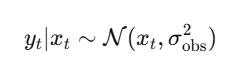
The Bootstrap Particle Filter
The algorithm maintains N “particles” - each one a hypothesis about the true probability and reweights them as data arrives:
1. INITIALIZE: Draw x_0^{(i)} ~ Prior  for i = 1,...,N
   Set weights w_0^{(i)} = 1/N

2. FOR each new observation y_t:
   a. PROPAGATE:  x_t^{(i)} ~ f( · | x_{t-1}^{(i)} )
   b. REWEIGHT:   w_t^{(i)} ∝ g( y_t | x_t^{(i)} )
   c. NORMALIZE:  w̃_t^{(i)} = w_t^{(i)} / Σ_j w_t^{(j)}
   d. RESAMPLE if ESS = 1/Σ(w̃_t^{(i)})² < N/2
Particle Filter for a Live Prediction Market
import numpy as np
from scipy.special import expit, logit  # sigmoid and logit

class PredictionMarketParticleFilter:
    """
    Sequential Monte Carlo filter for real-time event probability estimation.

    Usage during a live event (e.g., election night):
        pf = PredictionMarketParticleFilter(prior_prob=0.50)
        pf.update(observed_price=0.55)   # market moves on early returns
        pf.update(observed_price=0.62)   # more data
        pf.update(observed_price=0.58)   # partial correction
        print(pf.estimate())             # filtered probability
    """
    def __init__(self, N_particles=5000, prior_prob=0.5,
                 process_vol=0.05, obs_noise=0.03):
        self.N = N_particles
        self.process_vol = process_vol
        self.obs_noise = obs_noise

        # Initialize particles around prior
        logit_prior = logit(prior_prob)
        self.logit_particles = logit_prior + np.random.normal(0, 0.5, N_particles)
        self.weights = np.ones(N_particles) / N_particles
        self.history = []

    def update(self, observed_price):
        """Incorporate a new observation (market price, poll result, etc.)"""
        # 1. Propagate: random walk in logit space
        noise = np.random.normal(0, self.process_vol, self.N)
        self.logit_particles += noise

        # 2. Convert to probability space
        prob_particles = expit(self.logit_particles)

        # 3. Reweight: likelihood of observation given each particle
        log_likelihood = -0.5 * ((observed_price - prob_particles) / self.obs_noise)**2
        log_weights = np.log(self.weights + 1e-300) + log_likelihood

        # Normalize in log space for stability
        log_weights -= log_weights.max()
        self.weights = np.exp(log_weights)
        self.weights /= self.weights.sum()

        # 4. Check ESS and resample if needed
        ess = 1.0 / np.sum(self.weights**2)
        if ess < self.N / 2:
            self._systematic_resample()

        self.history.append(self.estimate())

    def _systematic_resample(self):
        """Systematic resampling - lower variance than multinomial."""
        cumsum = np.cumsum(self.weights)
        u = (np.arange(self.N) + np.random.uniform()) / self.N
        indices = np.searchsorted(cumsum, u)
        self.logit_particles = self.logit_particles[indices]
        self.weights = np.ones(self.N) / self.N

    def estimate(self):
        """Weighted mean probability estimate."""
        probs = expit(self.logit_particles)
        return np.average(probs, weights=self.weights)

    def credible_interval(self, alpha=0.05):
        """Weighted quantile-based credible interval."""
        probs = expit(self.logit_particles)
        sorted_idx = np.argsort(probs)
        sorted_probs = probs[sorted_idx]
        sorted_weights = self.weights[sorted_idx]
        cumw = np.cumsum(sorted_weights)
        lower = sorted_probs[np.searchsorted(cumw, alpha/2)]
        upper = sorted_probs[np.searchsorted(cumw, 1 - alpha/2)]
        return lower, upper

# --- Simulate election night ---
pf = PredictionMarketParticleFilter(prior_prob=0.50, process_vol=0.03)

# Incoming observations (market prices as new data arrives)
observations = [0.50, 0.52, 0.55, 0.58, 0.61, 0.63, 0.60,
                0.65, 0.70, 0.75, 0.80, 0.85, 0.90, 0.95]

print("Election Night Tracker:")
print(f"{'Time':>6}  {'Observed':>10}  {'Filtered':>10}  {'95% CI':>20}")
print("-" * 52)

for t, obs in enumerate(observations):
    pf.update(obs)
    ci = pf.credible_interval()
    print(f"{t:>5}h  {obs:>10.3f}  {pf.estimate():>10.3f}  ({ci[0]:.3f}, {ci[1]:.3f})")
Why is this better than just using the market price directly?
Because the particle filter smooths noise and propagates uncertainty.
When the market spikes from 0.65 on a single trade, the filter recognizes that the true probability might not have changed that much it tempers the update based on how volatile the observation process has been.
Part V: Three Variance Reduction Tricks That Stack
Before we leave Monte Carlo territory, here are three techniques that combine multiplicatively with everything above.
Free Symmetry
When the payoff function is monotone (which binary contracts always are higher prices mean higher probability of exceeding the strike), the variance reduction is guaranteed:

Typical reduction is around 50-75%. Zero extra computational cost beyond doubling the function evaluations (which you were going to do anyway).
Exploit What You Already Know
If you’re simulating a binary contract {S_T > K} under stochastic volatility (no closed form), use the Black-Scholes digital price p_{BS} (which has a closed form) as a control variate:
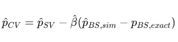
Divide and Conquer
Partition the probability space into JJ J strata, sample within each, combine. The variance is always ≤ crude MC (by the law of total variance), with maximum gain from Neyman allocation: nj∝ωjσj (oversample strata with high variance).
def stratified_binary_mc(S0, K, sigma, T, J=10, N_total=100_000):
    """
    Stratified MC for binary contract pricing.
    Strata defined by quantiles of the terminal price distribution.
    """
    n_per_stratum = N_total // J
    estimates = []

    for j in range(J):
        # Uniform draws within stratum [j/J, (j+1)/J]
        U = np.random.uniform(j/J, (j+1)/J, n_per_stratum)
        Z = norm.ppf(U)
        S_T = S0 * np.exp((-0.5*sigma**2)*T + sigma*np.sqrt(T)*Z)
        stratum_mean = (S_T > K).mean()
        estimates.append(stratum_mean)

    # Each stratum has weight 1/J
    p_stratified = np.mean(estimates)
    se_stratified = np.std(estimates) / np.sqrt(J)

    return p_stratified, se_stratified

p, se = stratified_binary_mc(S0=100, K=105, sigma=0.20, T=30/365)
print(f"Stratified estimate: {p:.6f} ± {se:.6f}")
Stack all three
Antithetic variates inside each stratum, with a control variate correction and you routinely achieve 100–500x variance reduction over crude MC. This is not optional in production. This is table stakes.
Part VI: Modeling What Correlation Matrices Can’t
The hierarchical Bayesian model implicitly encodes correlation through the shared national swing parameter.
But what about tail dependence - the tendency for extreme co-movements that don’t show up in linear correlation?
In 2008, the Gaussian copula’s failure to model tail dependence contributed to the global financial crisis. In prediction markets, the same issue arises: when one swing state has a surprise result, the probability that all swing states flip together is much higher than a Gaussian copula would predict.
Sklar’s Theorem

where C is the copula (the pure dependency structure) and F_i are the marginal CDFs. You can model each market’s marginal behavior separately, then glue them together with a copula that captures the dependency including in the tails.
The Tail Dependence Problem
Gaussian copula: Tail dependence λU=λL=0. Extreme co-movements are modeled as having zero probability.
This is catastrophically wrong for correlated prediction markets.
Student-t copula
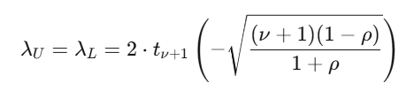
With ν=4 and ρ=0.6, tail dependence is approximately 0.18 -z an 18% probability that extreme co-movement occurs given one contract hits an extreme. Gaussian would say 0%.
Clayton copula: Lower tail dependence only (λL=2^−1/θ. When one prediction market crashes, others follow. No upper tail dependence.
Gumbel copula: Upper tail dependence only (λU=2−2^1/θ). Correlated positive resolutions.
Simulating Correlated Prediction Market Outcomes
import numpy as np
from scipy.stats import norm, t as t_dist

def simulate_correlated_outcomes_gaussian(probs, corr_matrix, N=100_000):
    """Gaussian copula no tail dependence."""
    d = len(probs)
    L = np.linalg.cholesky(corr_matrix)
    Z = np.random.standard_normal((N, d))
    X = Z @ L.T
    U = norm.cdf(X)
    outcomes = (U < np.array(probs)).astype(int)
    return outcomes

def simulate_correlated_outcomes_t(probs, corr_matrix, nu=4, N=100_000):
    """Student-t copula symmetric tail dependence."""
    d = len(probs)
    L = np.linalg.cholesky(corr_matrix)
    Z = np.random.standard_normal((N, d))
    X = Z @ L.T

    # Divide by sqrt(chi-squared / nu) to get t-distributed
    S = np.random.chisquare(nu, N) / nu
    T = X / np.sqrt(S[:, None])
    U = t_dist.cdf(T, nu)
    outcomes = (U < np.array(probs)).astype(int)
    return outcomes

def simulate_correlated_outcomes_clayton(probs, theta=2.0, N=100_000):
    """Clayton copula (bivariate) lower tail dependence."""
    # Marshall-Olkin algorithm
    V = np.random.gamma(1/theta, 1, N)
    E = np.random.exponential(1, (N, len(probs)))
    U = (1 + E / V[:, None])**(-1/theta)
    outcomes = (U < np.array(probs)).astype(int)
    return outcomes


# --- Compare tail behavior ---
probs = [0.52, 0.53, 0.51, 0.48, 0.50]  # 5 swing state probabilities
state_names = ['PA', 'MI', 'WI', 'GA', 'AZ']

corr = np.array([
    [1.0, 0.7, 0.7, 0.4, 0.3],
    [0.7, 1.0, 0.8, 0.3, 0.3],
    [0.7, 0.8, 1.0, 0.3, 0.3],
    [0.4, 0.3, 0.3, 1.0, 0.5],
    [0.3, 0.3, 0.3, 0.5, 1.0],
])

N = 500_000

gauss_outcomes = simulate_correlated_outcomes_gaussian(probs, corr, N)
t_outcomes = simulate_correlated_outcomes_t(probs, corr, nu=4, N=N)

# P(sweep all 5 states)
p_sweep_gauss = gauss_outcomes.all(axis=1).mean()
p_sweep_t = t_outcomes.all(axis=1).mean()

# P(lose all 5 states)
p_lose_gauss = (1 - gauss_outcomes).all(axis=1).mean()
p_lose_t = (1 - t_outcomes).all(axis=1).mean()

# If independent
p_sweep_indep = np.prod(probs)
p_lose_indep = np.prod([1-p for p in probs])

print("Joint Outcome Probabilities:")
print(f"{'':>25}  {'Independent':>12}  {'Gaussian':>12}  {'t-copula':>12}")
print(f"{'P(sweep all 5)':>25}  {p_sweep_indep:>12.4f}  {p_sweep_gauss:>12.4f}  {p_sweep_t:>12.4f}")
print(f"{'P(lose all 5)':>25}  {p_lose_indep:>12.4f}  {p_lose_gauss:>12.4f}  {p_lose_t:>12.4f}")
print(f"\nt-copula increases sweep probability by {p_sweep_t/p_sweep_gauss:.1f}x vs Gaussian")
This is the exact reason the Gaussian copula failed in 2008 and would fail again for prediction market portfolios.
The t-copula with v = 4 routinely shows 2–5x higher probability of extreme joint outcomes.
If you’re trading correlated prediction market contracts without modeling tail dependence, you’re running a portfolio that will blow up in exactly the scenarios that matter most.
Vine Copula
For d>5 contracts, bivariate copulas are insufficient. Vine copulas decompose the dd d-dimensional dependency into d(d−1)/2 bivariate conditional copulas arranged in a tree structure:
-
C-vine (star): One central event drives everything (e.g., presidential winner → all policy markets)
-
D-vine (path): Sequential dependencies (e.g., primary results flow into general election)
-
R-vine (general graph): Maximum flexibility
build maximum spanning trees ordered by ∣τKendall∣, select pair-copula families via AIC, estimate sequentially. Implementations: pyvinecopulib (Python), VineCopula (R).
Part VII: Agent-Based Simulation
Everything so far assumes you know the data-generating process and just need to simulate it.
But prediction markets are populated by heterogeneous agents - informed traders, noise traders, market makers, and bots whose interactions produce emergent dynamics that no closed-form SDE can capture.
The Zero-Intelligence Revelation
Markets can be efficient even when every single trader is completely irrational.
Gode & Sunder (1993) showed that zero-intelligence agents - traders who submit random orders subject only to budget constraints achieve near-100% allocative efficiency in a continuous double auction.
Farmer, Patelli & Zovko (2005) extended this to limit order books.
This explained 96% of cross-sectional spread variation on the London Stock Exchange. One parameter. 96%.
Agent-Based Prediction Market Simulator
import numpy as np
from collections import deque

class PredictionMarketABM:
    """
    Agent-based model of a prediction market order book.

    Agent types:
    - Informed: know the true probability, trade toward it
    - Noise: random trades
    - Market maker: provides liquidity around current price
    """
    def __init__(self, true_prob, n_informed=10, n_noise=50, n_mm=5):
        self.true_prob = true_prob
        self.price = 0.50  # initial price
        self.price_history = [self.price]

        # Order book (simplified as bid/ask queues)
        self.best_bid = 0.49
        self.best_ask = 0.51

        # Agent populations
        self.n_informed = n_informed
        self.n_noise = n_noise
        self.n_mm = n_mm

        # Track metrics
        self.volume = 0
        self.informed_pnl = 0
        self.noise_pnl = 0

    def step(self):
        """One time step: randomly select an agent to trade."""
        total = self.n_informed + self.n_noise + self.n_mm
        r = np.random.random()

        if r < self.n_informed / total:
            self._informed_trade()
        elif r < (self.n_informed + self.n_noise) / total:
            self._noise_trade()
        else:
            self._mm_update()

        self.price_history.append(self.price)

    def _informed_trade(self):
        """Informed trader: buy if price < true_prob, sell otherwise."""
        signal = self.true_prob + np.random.normal(0, 0.02)  # noisy signal

        if signal > self.best_ask + 0.01:  # buy
            size = min(0.1, abs(signal - self.price) * 2)
            self.price += size * self._kyle_lambda()
            self.volume += size
            self.informed_pnl += (self.true_prob - self.best_ask) * size
        elif signal < self.best_bid - 0.01:  # sell
            size = min(0.1, abs(self.price - signal) * 2)
            self.price -= size * self._kyle_lambda()
            self.volume += size
            self.informed_pnl += (self.best_bid - self.true_prob) * size

        self.price = np.clip(self.price, 0.01, 0.99)
        self._update_book()

    def _noise_trade(self):
        """Noise trader: random buy/sell."""
        direction = np.random.choice([-1, 1])
        size = np.random.exponential(0.02)
        self.price += direction * size * self._kyle_lambda()
        self.price = np.clip(self.price, 0.01, 0.99)
        self.volume += size
        self.noise_pnl -= abs(self.price - self.true_prob) * size * 0.5
        self._update_book()

    def _mm_update(self):
        """Market maker: tighten spread toward current price."""
        spread = max(0.02, 0.05 * (1 - self.volume / 100))
        self.best_bid = self.price - spread / 2
        self.best_ask = self.price + spread / 2

    def _kyle_lambda(self):
        """Price impact parameter."""
        sigma_v = abs(self.true_prob - self.price) + 0.05
        sigma_u = 0.1 * np.sqrt(self.n_noise)
        return sigma_v / (2 * sigma_u)

    def _update_book(self):
        spread = self.best_ask - self.best_bid
        self.best_bid = self.price - spread / 2
        self.best_ask = self.price + spread / 2

    def run(self, n_steps=1000):
        for _ in range(n_steps):
            self.step()
        return np.array(self.price_history)


# --- Simulation ---
np.random.seed(42)

# Scenario: true probability is 0.65, market starts at 0.50
sim = PredictionMarketABM(true_prob=0.65, n_informed=10, n_noise=50, n_mm=5)
prices = sim.run(n_steps=2000)

print("Agent-Based Prediction Market Simulation")
print(f"True probability:   {sim.true_prob:.2f}")
print(f"Starting price:     0.50")
print(f"Final price:        {prices[-1]:.4f}")
print(f"Price at t=500:     {prices[500]:.4f}")
print(f"Price at t=1000:    {prices[1000]:.4f}")
print(f"Total volume:       {sim.volume:.1f}")
print(f"Informed P&L:       ${sim.informed_pnl:.2f}")
print(f"Noise trader P&L:   ${sim.noise_pnl:.2f}")
print(f"Convergence error:  {abs(prices[-1] - sim.true_prob):.4f}")
How fast prices converge depends on the ratio of informed to noise traders, how market maker spread responds to information flow, and why the informed traders extract profit at noise traders expense.
Part VIII: The Production Stack
Here’s the complete system, from market data to trade execution:
-
LAYER 1: DATA INGESTION - WebSocket feed from Polymarket CLOB API (real-time prices, volumes) - News/poll feeds (NLP-processed into probability signals) - On-chain event data (Polygon)
-
LAYER 2: PROBABILITY ENGINE - Hierarchical Bayesian model (Stan/PyMC) state-level posteriors - Particle filter real-time updating on new observations - Jump-diffusion SDE path simulation for risk management - Ensemble: weighted average of model outputs
-
LAYER 3: DEPENDENCY MODELING - Vine copula pairwise dependencies between contracts - Factor model shared national/global risk factors - Tail dependence estimation via t-copula
-
LAYER 4: RISK MANAGEMENT - EVT-based VaR and Expected Shortfall - Reverse stress testing identify worst-case scenarios - Correlation stress what if state correlations spike? - Liquidity risk order book depth monitoring
-
LAYER 5: MONITORING - Brier score tracking (are we calibrated?) - P&L attribution (which model component added value?) - Drawdown alerts - Model drift detection
References
-
Dalen (2025). “Toward Black-Scholes for Prediction Markets.” arXiv:2510.15205
-
Saguillo et al. (2025). “Unravelling the Probabilistic Forest: Arbitrage in Prediction Markets.” arXiv:2508.03474
-
Madrigal-Cianci et al. (2026). “Prediction Markets as Bayesian Inverse Problems.” arXiv:2601.18815
-
Farmer, Patelli & Zovko (2005). “The Predictive Power of Zero Intelligence.” PNAS
-
Gode & Sunder (1993). “Allocative Efficiency of Markets with Zero-Intelligence Traders.” JPE
-
Kyle (1985). “Continuous Auctions and Insider Trading.” Econometrica
-
Glosten & Milgrom (1985). “Bid, Ask, and Transaction Prices.” JFE
-
Hoffman & Gelman (2014). “The No-U-Turn Sampler.” JMLR
-
Merton (1976). “Option Pricing When Underlying Stock Returns Are Discontinuous.” JFE
-
Linzer (2013). “Dynamic Bayesian Forecasting of Presidential Elections.” JASA
-
Gelman et al. (2020). “Updated Dynamic Bayesian Forecasting Model.” HDSR
-
Aas, Czado, Frigessi & Bakken (2009). “Pair-Copula Constructions of Multiple Dependence.” Insurance: Mathematics and Economics
-
Wiese et al. (2020). “Quant GANs: Deep Generation of Financial Time Series.” Quantitative Finance
-
Kidger et al. (2021). “Neural SDEs as Infinite-Dimensional GANs.” ICML